The Importance of Weather Variations in a Quantitative Risk Analysis

By
Jeffery Marx and John Cornwell

Presented at Presented At Mary Kay O’Conner Process Safety Center 2008 International Symposium October 28-29, 2008 Texas A&M University College Station, Texas

Abstract

As more and more quantitative risk analyses (QRAs) are performed for petrochemical facilities around the world, the variety of techniques used in these analyses continually expands. Although the emphasis is often placed on risk’s two constituents, consequence and probability, many of the contributing elements get marginalized, or even lost in the analysis. One such element is the weather data. Changes in wind speed and atmospheric stability affect the size and extent of impact zones, while the different wind directions modify how the impacts are mapped in the area surrounding each release point when creating risk contours. Weather data is often defined by the three variables (wind speed, atmospheric stability, and wind direction), and is site-specific in nature, with definable probabilities for each triplet combination. Many QRA studies shortcut the quantitative nature of an analysis by condensing the weather data into a small number of combinations, with unpredictable results. By utilizing robust risk mapping techniques, it can be demonstrated that risk contours may be critically dependent on the number of wind speed/stability/direction combinations employed in the analysis. This paper will also demonstrate how a risk assessment can arrive at different conclusions based on the level of weather data detail applied in the analysis.

---

Text

Introduction

In the petrochemical industry, the use of quantitative risk analysis (QRA) is becoming more frequent. Because of increasing prevalence, many process safety specialists are beginning to understand the value of QRA. Although QRA is gaining higher levels of acceptance in the industry, there remains a con­siderable degree of misunderstanding about what constitutes an accurate QRA.

By definition, a QRA is a quantitative analysis. This means that all aspects of the analysis should be quantified to the extent possible. Quantification means not only assigning a numeric value to each part of the calculations, but evaluating the potential range of each variable. For some variables, such as release orientation, a conservative assumption (e.g., all releases are oriented horizontally in the direction the wind is blowing) can serve to simplify the analysis while at the same time calculating a risk value that results in an overprediction of the true risk. For other variables, such as weather conditions, this may not be possible.

Weather Variations

In the real world, the variations of the weather are infinite. But, as measurements are taken, these variations can be classified into groups that reasonably represent the spread of measured values. After collecting a set of measurements spanning at least one year, a set of data can be generated that represents how often certain conditions occur. A probabilistic data set is generated by comparing the number of occurrences for each combination of measured variables to the total number of observations. This set of data is specific to the location at which it is measured.

The most common weather variables used in consequence and risk analysis are wind speed, wind direction, and atmospheric stability. Probabilistic data involving these three variables is often available for specific locations. In the United States, the National Climactic Data Center in Asheville, North Carolina, maintains a database of weather data for thousands of sites across the country. One form of such data is the stability array (STAR) tabulations. Developed over 30 years ago, the STAR format provides a compact probabilistic representation of the wind speed, stability, and wind direction triplets measured at a site. The wind direction is divided into 16 compass directions, while the wind speed is put into six categories. Atmospheric stability is classified by the Pasquill-Gifford system into six or seven categories, designated with letters. Stability A is the most unstable atmosphere, D is neutral, and F or G is the most stable. Because most considerations of stability only include six categories, G stability data is often collapsed into the F category.

The most common way to display weather data is with a wind rose. This format shows 16 wind directions and wind speed classes as a function of the percentage of time, per year, that each combination occurs. This, of course, does not include atmospheric stability. Stability can be included through the use of multiple wind roses, one for each stability class, and one for all stability classes combined. An example wind rose for Corpus Christi, Texas, for all stability classes, is shown in Figure 1.

An alternate method of showing this data is through the use of a wind speed/stability matrix. This format is demonstrated in Figure 2, for the Corpus Christi data. The bold line in Figure 2 surrounds the wind speed/stability combinations that occur at Corpus Christi. The numerical value in each matrix element is the fraction of the time, per year, that the combination of wind speed and stability occurs, for all wind directions. The wind speed values on the left of the matrix are the average wind speed value, in meters per second, for that category. For example, the 2^nd STAR category is defined as 4-6 knots. This category is assumed to include wind speeds between 4.0 knots and 6.9 knots (the 3^rd category is defined as 7-10 knots). The average value, 5.5 knots, is equal to 2.83 m/s or 6.3 mph. Within the A stability classification, this wind speed has an annual probability of 0.00258, or 0.258% of the time.

Risk Analysis Methodology

A QRA consists of four fundamental steps:

• Hazard identification and scenario selection
• Consequence analysis
• Probability analysis
• Risk mapping

Using the physical and chemical properties of the materials in the facility, and the conditions in which they are processed, the potential hazards can be identified. These normally include toxic vapor clouds, torch fires, pool fires, flash fires, vapor cloud explosions, and BLEVE fireballs.

The selection of potential release sources of flammable and toxic materials is based on process information, accident history, and engineering analysis. Using the release conditions (composition, pressure, temperature, hole size, inventory, etc.) and varying the weather conditions (wind speed and atmospheric stability), each specific scenario is modeled to produce a unique set of hazard impact zones.

The frequency with which a given failure case is expected to occur can be estimated by using a combination of historical experience (databases), service factors, and engineering judgment. This is most often accomplished by using single component failures (e.g., pipe rupture) available in industrial failure rate data bases. For multiple component failures (e.g., failure of an automatic system for preventing an uncontrolled release from a cargo transfer arm), fault tree analysis (FTA) techniques can be used.

The risk mapping portion of the analysis incorporates the probability of each failure, the probability of the weather conditions (including wind direction) and the hazard zone maps. When each hazard zone is combined with its respective probabilities and mapped at the correct location, the result is a prediction of the frequency at which specific impact levels can affect locations around the release points, also known as risk contours.

Example Facility

As an example, consider an LPG recovery unit within a larger hydrocarbon processing facility. The system consists of several distillation towers and associated equipment. For brevity, the extent of the analysis was constrained to this process unit. A depiction of the unit is shown in Figure 3.

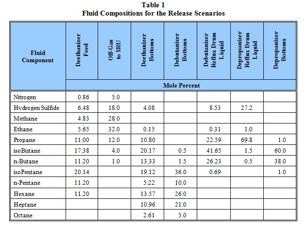
Seven basic accident scenarios were chosen from this system, as denoted by the stars in Figure 3. Five of the seven scenarios contain hydrogen sulfide (H₂S), and all scenarios are flammable. Thus, the hazards associated with this process unit are toxic vapor dispersion, torch fires, pool fires, flash fires (flammable vapor dispersion), and vapor cloud explosions. The fluid compositions for the seven scenarios are listed in Table 1.

In a QRA, the set of endpoints used in the analysis requires time-dependent fatality values for all hazard types. This approach is necessary if multiple hazard types are to be equally evaluated when combined to predict overall risk. In addition, nearly all risk acceptability criteria are based on the annual probability of fatalities. For flammable vapor dispersion (representing flash fires), the lower flammable limit (LFL) was defined as the endpoint. It is assumed that any person within the flammable cloud at the time it is ignited will suffer fatal burn injuries, and outside this area, there will be no fatal impact. Toxic vapor dispersion, vapor cloud explosion overpressure, and fire radiation calculations used probit equations to determine the endpoints. For fire radiation impacts, a 30-second exposure was assumed. Toxic gas exposure times were varied based on the duration of the release.

For the consequence modeling calculations presented in this paper, the CANARY by Quest® computer software hazards analysis package was used to produce hazard zones for the flammable and toxic impacts associated with each failure case. The models that are used account for:

• Mixture thermodynamics
• Release conditions
• Aerosol formation and post-release phase separation
• Ambient weather conditions (wind speed, air temperature, humidity, atmospheric stability)
• Effects of the local terrain (diking, obstacles)

To demonstrate the importance of weather data, several QRAs were run for this example process unit. The base case used the Corpus Christi weather data presented above, while others used variations of that data. The facility layout, list of accident scenarios, equipment counts (probabilities), endpoints, and consequence modeling were all kept constant throughout the QRA studies. The only variable modified during the analysis was the weather data.

Base Case

The base case scenario involved the seven accident locations presented in the previous section and an evaluation of three hole sizes: ruptures (full pipe break), punctures (1-inch diameter hole) and leaks (1/4-inch diameter hole). For each of these 21 releases, flammable dispersion modeling was performed for the 21 valid wind speed/stability combinations. For fire radiation cases (torch fires and pool fires), atmospheric stability is not an important variable, so each fire calculation for a specific hole size requires only six calculations, one for each wind speed category.

Quest’s risk mapping software has the ability to map the hazard zones in 64 wind directions based on the 16 provided in the weather data. This is accomplished by inserting three wind directions between each of the original 16, and adjusting the probability of each wind direction. Applying this method results in a more representa­tive risk prediction. When using this approach, the risk mapping involves 64 wind directions, 21 wind speed/stability combinations, and three hole sizes for each release scenario, for a total of 4,032 unique mappings for each vapor dispersion outcome and 1,152 for each torch fire or pool fire outcome.

The results from this effort, for the seven release scenarios identified in the example facility, are the individual risk contours shown in Figure 4. These contours are derived from the raw data output from the risk mapping and have not been “smoothed” for presentation; they have been left in their natural state to fully demonstrate the results.

These contours predict the annual risk of being fatally affected by all releases from the LPG recovery unit considered in this study. For example, a risk contour denoted by 10^-6 indicates that on that contour, there is one chance in one million, per year, of being fatally affected by a release from the LPG unit. The contours include impacts from all weather conditions, all three hole sizes evaluated, and all of the potential hazards (flash fires, torch fires, pool fires, vapor cloud explosions, and toxic gases). These contours also assume that the risk at any one location is based on 100% occupancy. This means that an individual would have to remain at one location 365 days/year and 24 hours/day to be exposed to the level of risk predicted by a contour passing through that location.

Variation 1

The first variation on the risk analysis involved constraining the analysis to 16 wind directions. This set of calculations did not change anything in the Corpus Christi weather data file; it simply did not sub-divide the 16 wind directions into 64 as in the base case. The raw risk contours for Variation 1 are shown in Figure 5.

As seen in Figure 5, the outer risk contours (those defined by the largest impacts in the analysis) demonstrate an effect associated with using a reduced number of wind directions. Although the furthest extent of the contours does not change appreciably, there are “holes” created in the edges of the contours that alter the specific impact predicted at a location.

Variation 2

This variation of the weather data condensed the Corpus Christi weather data into six wind speed/stability combinations, one for each stability class. For each stability class, the frequencies of occurrence were summed into the single category used in the analysis. The six categories and their respective frequencies are:

Wind Speed Stability Annual Probability

• 1.03 m/s A 0.00416
• 2.83 m/s B 0.04543
• 10.36 m/s C 0.11548
• 4.63 m/s D 0.56516
• 2.83 m/s E 0.12876
• 1.03 m/s F 0.14102

In addition, the calculations for Variation 2 used only 16 wind directions, as in Variation 1. This weather data set represents an attempt to simplify the data while representing all six stabilities. The results of this analysis are shown in Figure 6.

A comparison of Figure 6 to Figures 5 and 4 shows that the extent of the risk contours has diminished. This is a direct result of not modeling several of the wind speed/stability combinations that define the furthest extent of some of the hazards.

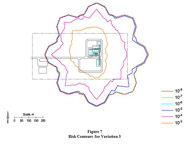
Variation 3

The final variation on the weather data is based on a minimal data set. This involved two wind speed/
stability combinations (1.03 m/s and F; 4.63 m/s and D) and only 8 wind directions. Probability values were assigned to these categories by condensing all the probabilities of wind speed classes within the E and F stabilities into the 1.03/F case, and condensing the probabilities of all remaining combinations in the original data set into the 4.63/D case. Although this is obviously an over-simplification of the weather data, there have been studies, labeled as QRAs, that applied this level of detail to the weather data. The risk contours for Variation 3 are shown in Figure 7.

Concluding Remarks

The obvious conclusion from this study is that the detail applied in the weather conditions matters a great deal in the prediction of the risk. The following observations were made:

• The most minor change, mapping 16 base wind directions instead expanding to 64, results in less realistic risk contours which have similar extents. Because the weather data is provided with 16 directions, the use of 64 directions in the mapping software is an improvement that provides a modest improvement in risk contour quality.
• The exclusion of a significant number of wind speed/stability combinations results in risk contours that do not extend as far from the source area as in a full analysis, and thus could present an underprediction of risk.
• Representing the weather data with a small set of combinations (2 wind speed/stability combi­nations and 8 wind directions as used in Variation 3) significantly reduces the accuracy of the risk analysis, providing a sizeable underprediction of the risk posed to the surrounding area.

A comparison of the base case and three variations is shown in Figure 8, using the 1.0 x 10^-6 risk level as the level of interest (10^-6 is a risk level frequently referenced as the threshold of acceptability for risk to the public).

Differences in the risk predictions are further demonstrated by evaluating the area within a specific risk contour. Calculations of the area covered by the 10^-6 contours for the base case and each variation are presented in Table 2.

Although this paper did not evaluate societal risk, the predicted risk contours show the potential to miss certain specific areas (such as potential populated sites) during the mapping, which would again result in an underprediction of risk in the f/N calculations.Some of the variations examined in this paper may not be as important for near field hazards, such as torch fires, pool fires, or explosions. The correct representation of weather is important for flash fire hazards (as defined by the LFL), and critically important for toxic gas dispersion. As demonstrated by Table 2 and the risk contours in Figure 8, there is a significant potential for underestimating risk when poor weather data are applied in a risk analysis.

Table 2

Area Coverage for the 10-6 Contours

Scenario	Area [m2] covered	% underprediction, by area
Base Case	613,318	0.0%
Variation 1	574,878	6.3%
Variation 2	443,351	27.7%
Variation 3	332,028	45.9%